The bathtub curve
How failure rates vary throughout an asset’s lifespan: and how to use that data to guide maintenance choices.

Different failure mechanisms need different responses.
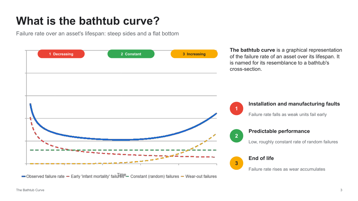
The bathtub curve represents a conceptual failure hazard pattern: it declines early in a product’s life, remains roughly steady during a middle phase, and rises again as wear-out mechanisms develop. It serves as a helpful hypothesis for assessment: not a universal lifecycle applicable to all machines.
This guide follows the provided slides, detailing the mathematics, evidence, pump example, and connections to predictive maintenance. The original images remain intact, with added explanations in the text regarding hazard, confidence intervals, and competing risks.
The three phases at a glance
| Pattern | Weibull shape | Questions for maintenance |
|---|---|---|
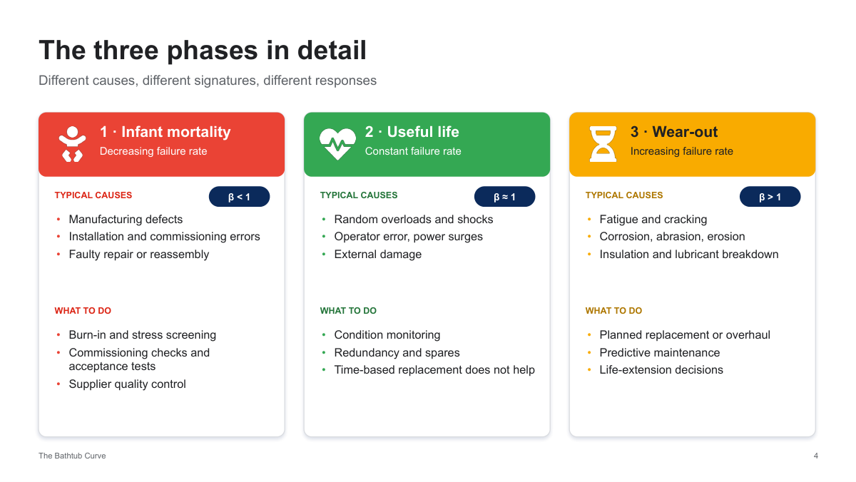
| Decreasing hazard | β < 1 | Are defects, installation or repairs driving early failures? |
| Constant hazard | β = 1 | Can monitoring, redundancy or spares reduce consequences? |
| Increasing hazard | β > 1 | Does planned intervention outperform waiting or monitoring? |
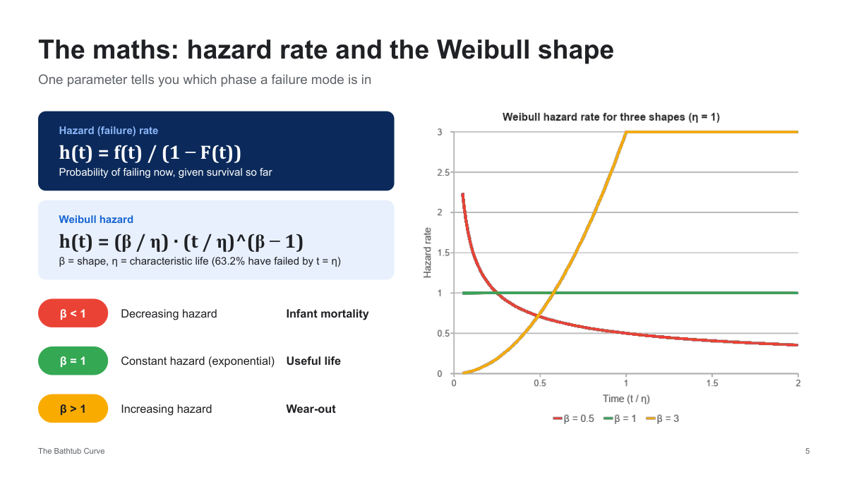
These β values correspond to a fitted two-parameter Weibull model. Capturing a complete bathtub curve necessitates a more complex or piecewise model, or a suitable combination of failure mechanisms.
Browse all 17 slides
01 · The bathtub curve 02 · From a familiar chart to practical decisions
 03 · What the curve actually shows
 04 · Three phases, three responses
 05 · Hazard rate and Weibull shape
 06 · Where reliability analysis helps
 07 · When to use the model cautiously
 08 · Hard-drive evidence is cohort-specific
 09 · Six patterns, not one universal law
 10 · Match the strategy to the mechanism
 11 · Build the curve from complete records
 12 · Interpret the fitting example carefully
 13 · Three pump modes and different actions
 14 · Combine reliability statistics with AI
 15 · Common misconceptions
 16 · Reliability metrics in context
 17 · Use the curve as a testable model
Understand the curve and its mathematics
The bathtub curve
The bathtub curve illustrates how the failure hazard of an asset population varies over time: initially high risk, followed by a stable middle phase, and finally a rising wear-out risk. It links reliability assessment with maintenance scheduling and predictive AI.
From a familiar chart to practical decisions
The deck addresses the curve, hazard and Weibull mathematics, applications, historical evidence, fitting workflows, and maintenance decisions. Its purpose is to evaluate the pattern using asset data instead of presuming it is universally applicable.
What the curve actually shows
The vertical axis represents the failure hazard for surviving units, rather than the cumulative failure probability. Early defects can cause a decreasing hazard, random failure mechanisms tend to result in an approximately constant hazard, and degradation leads to an increasing hazard. Not all assets show all three phases.
Three phases, three responses
Initial failures highlight the need for improved manufacturing, installation, commissioning, and well-founded screening. Ongoing age-related risk supports consequence-focused monitoring, redundancy, or allowing run-to-failure. Growing hazard levels may warrant planned interventions when justified by economic factors and failure mechanisms.
Hazard rate and Weibull shape
The hazard function is h(t) = f(t) / S(t), with S(t) = 1 − F(t). In the case of a two-parameter Weibull, h(t) = (β/η)(t/η)^(β−1): when β is less than one, the hazard decreases; when β equals one, the hazard remains constant; and when β is greater than one, the hazard increases. A single two-parameter Weibull cannot generate the complete bathtub-shaped hazard.
Applications, limits and historical patterns
Where reliability analysis helps
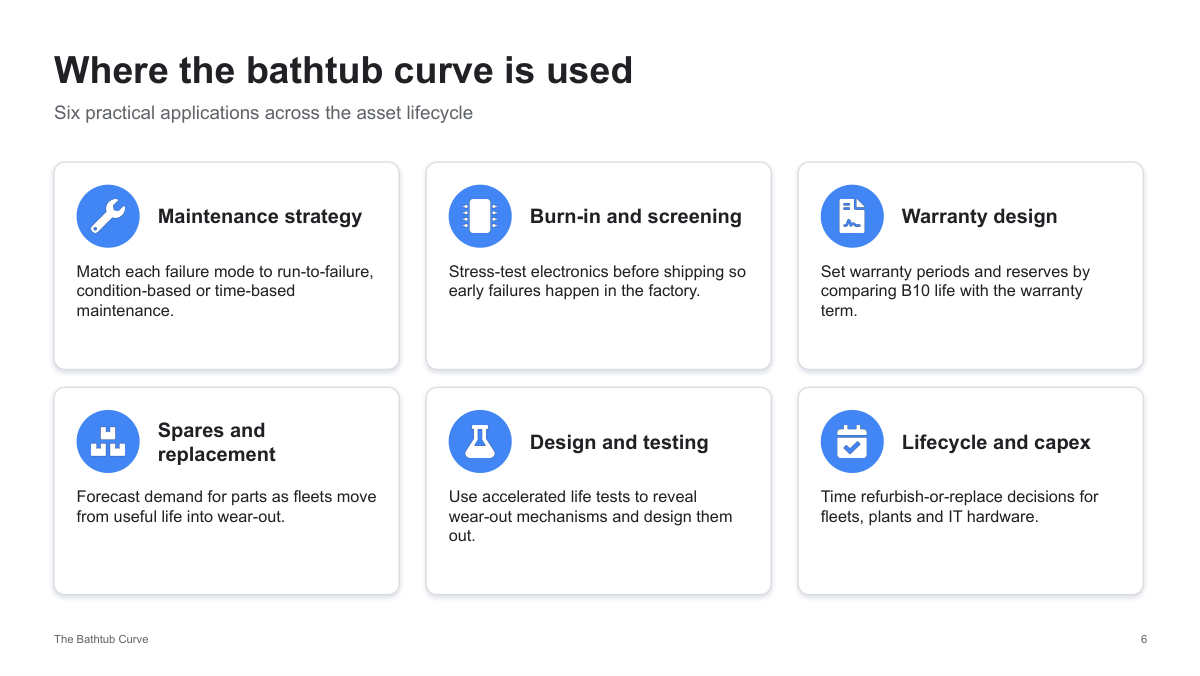
Applications encompass maintenance selection, screening, warranty reserves, spare parts forecasting, accelerated testing, and replacement planning. Decisions ought to integrate failure-mode data with consequences, uncertainty, and overall cost, rather than depend solely on a single curve or percentile.
When to use the model cautiously
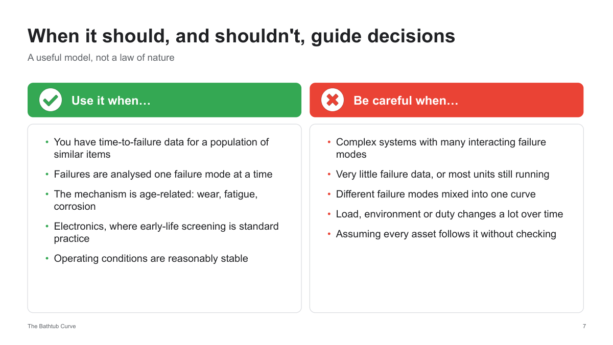
Examine similar units and identify failure mechanisms. Infrequent events, variable loads, combined environments, repairs, and interacting factors can mask aging effects. Confirm the model’s accuracy under real operating conditions prior to using its forecasts for a different fleet.
Hard-drive evidence is cohort-specific
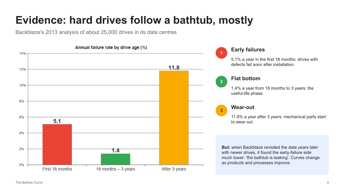
The deck references Backblaze’s historical 2013 annualized failure rates: 5.1% in the first 18 months, 1.4% between 18 months and three years, and 11.8% from three to four years. These figures represent past fleet data, not current forecasts for individual drives. Subsequent Backblaze analyses reveal that the failure rate patterns vary depending on product type and operating timeframe.
Six patterns, not one universal law
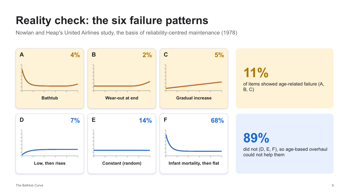
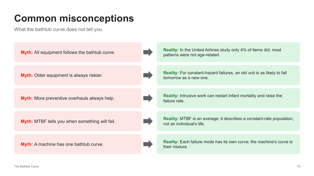
The presentation replicates traditional airline reliability patterns along with their historical proportions, including a 4% bathtub category. These percentages pertain specifically to that study context and should not be applied universally to all equipment. Limited age dependence does not diminish the importance of inspections or other maintenance based on consequence.
From fleet records to maintenance strategy
Match the strategy to the mechanism
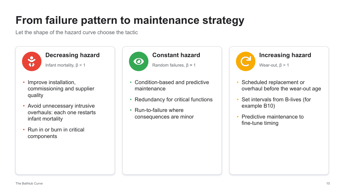
To reduce hazard, examine defects and minimize unnecessary intrusive activities. For a constant age hazard, assess condition data, redundancy, and potential consequences. When hazard increases with age, weigh planned replacement against inspection and condition-based maintenance. The age pattern of a failure mode serves as one factor in decision-making, not the whole policy.
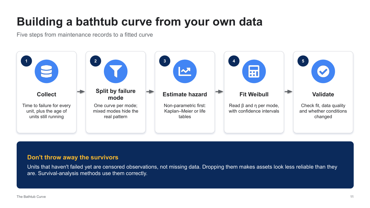
Build the curve from complete records
Gather exposure time, event status, failure cause, and operating context, including units that remain operational. Divide into suitable cohorts, estimate survival or cumulative hazard, fit potential models, and perform validation. Kaplan–Meier estimates survival; however, estimating instantaneous hazard needs an additional approach rather than directly extracting it from a survival curve.
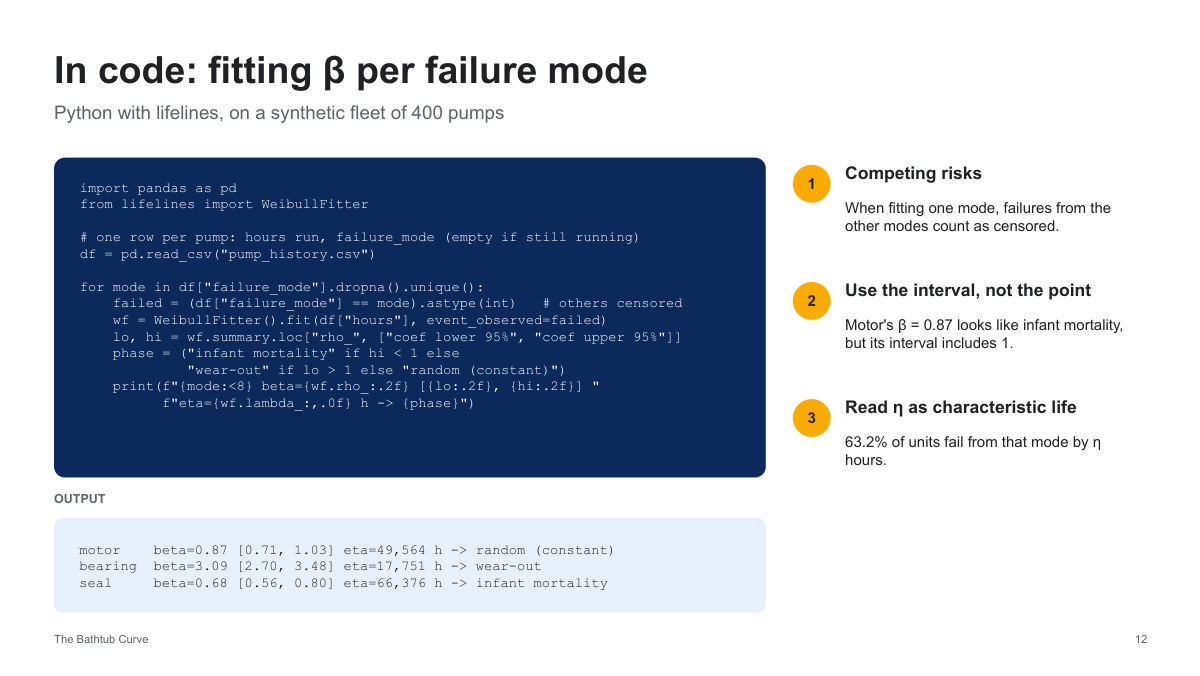
Interpret the fitting example carefully
The slide’s lifelines example applies mode-specific Weibull models to a synthetic pump fleet. Considering other failure modes as censored enables cause-specific hazard analysis within the model’s framework. However, it does not equate 1 − S for the fitted mode to the actual cumulative incidence in the presence of competing risks. A β confidence interval including one indicates that a constant hazard is still consistent with the data, though not conclusively established.
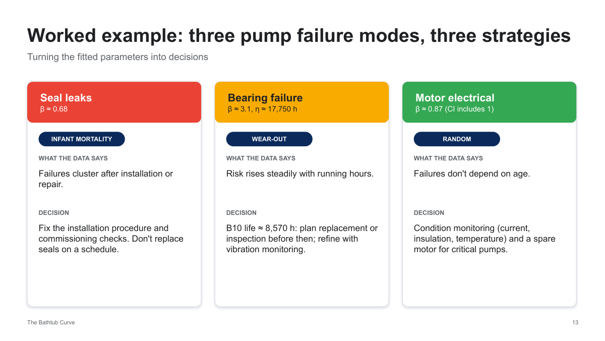
Three pump modes and different actions
The illustrative seal estimate indicates a decreasing hazard, while the bearing estimate indicates an increasing hazard; the motor interval, however, does not clarify the direction. With β = 3.09 and η = 17,751 hours, the fitted Weibull B10 is approximately 8,570 hours. This represents a model percentile, not a mandatory replacement time or a competing-risk incidence measure.
AI, misconceptions and reliability metrics
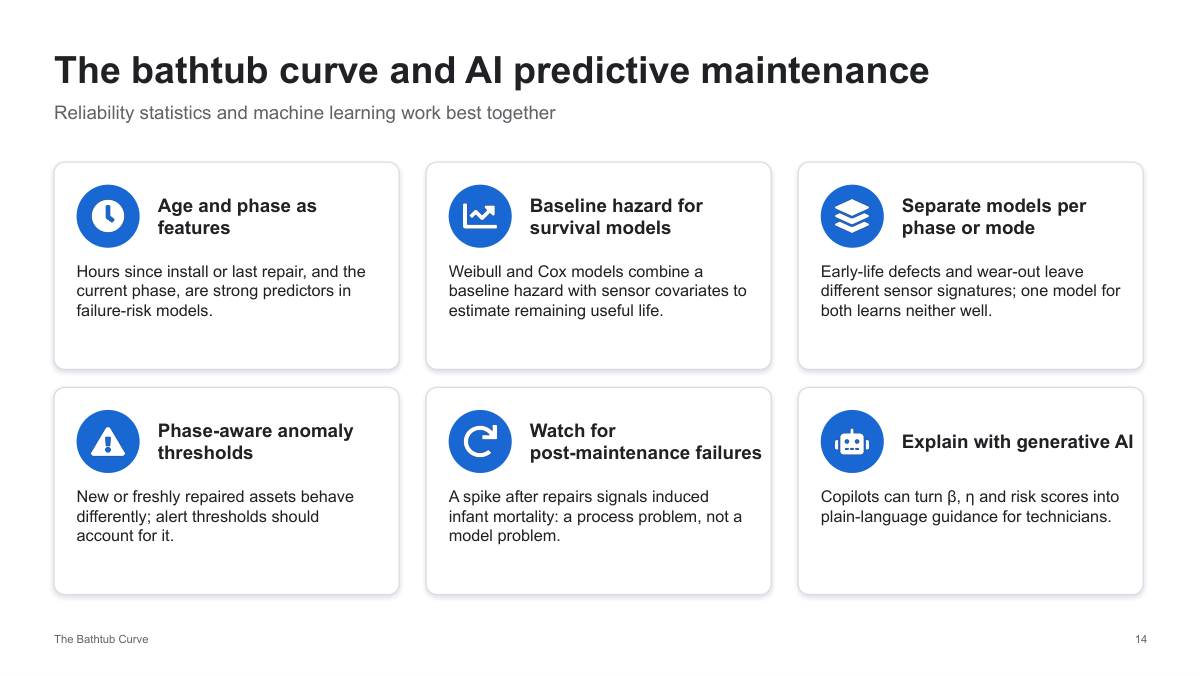
Combine reliability statistics with AI
Age, repair history, duty, and sensor data can enhance survival and failure-risk models once their predictive accuracy is confirmed. Models should be calibrated according to failure mechanisms and operational conditions. Generative AI can provide explanations for estimates, but maintenance decisions must stay grounded in engineering evidence and authorized protocols.
Common misconceptions
Not all equipment exhibits a bathtub curve, and age by itself does not dictate risk. Intrusive maintenance may cause defects. MTBF and MTTF represent averages rather than specific failure times; MTTF can also be defined for lifetime distributions with nonconstant hazard rates. When multiple failure modes compete, a detailed system model is necessary.
Reliability metrics in context
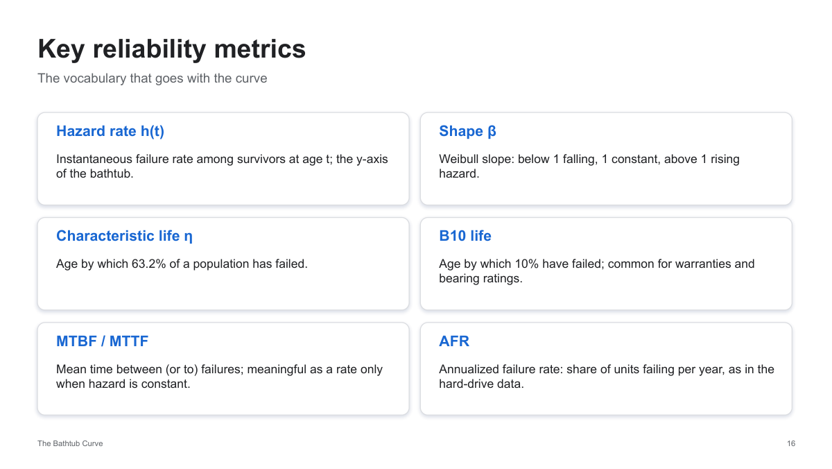
Hazard is an instantaneous rate measured in units of inverse time. In a two-parameter Weibull lifetime model, η represents the 63.2nd percentile of failure, while B10 denotes the 10th percentile. MTBF refers to the intervals between failures in repairable systems, whereas MTTF pertains to the time until failure. AFR is an annualized rate normalized by exposure and is not necessarily the probability that a unit fails within a year.
Use the curve as a testable model
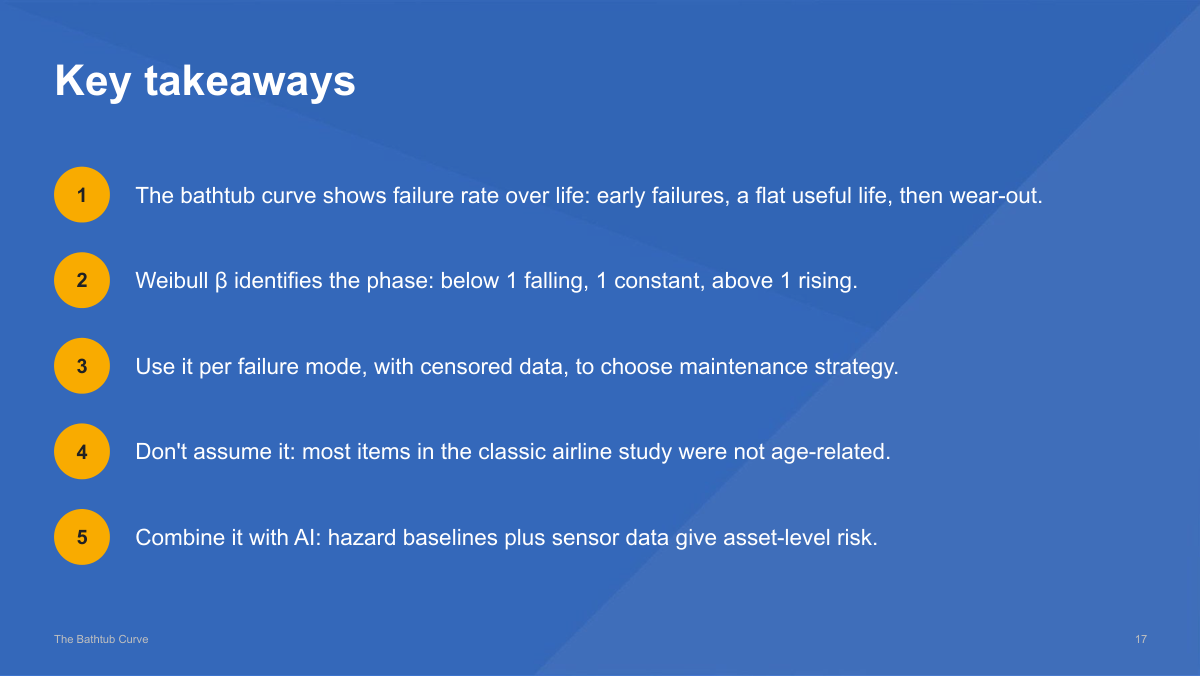
Determine the mechanism, retain censored data, measure uncertainty, and choose a maintenance approach based on both risk and impact. Integrate age-related reliability models with verified condition information, and reevaluate assumptions whenever there are changes in the fleet, operating conditions, or repair procedures.
Bathtub curve FAQ
What is the bathtub curve?
The bathtub curve illustrates how the failure hazard of an asset population varies over time: initially high risk, followed by a stable middle phase, and finally a rising wear-out risk. It links reliability assessment with maintenance scheduling and predictive AI.
What does Weibull beta mean?
In a two-parameter Weibull model, β < 1 indicates decreasing hazard, β = 1 constant hazard, and β > 1 increasing hazard. One such model represents a monotonic phase, not the entire bathtub.
Does every asset follow this pattern?
No. Different failure mechanisms, population makeup, operating conditions, and maintenance history result in varying patterns. Validate the model using similar asset data.
What is B10 life?
B10 represents the time at which the fitted lifetime model estimates that 10% of units have failed. For a two-parameter Weibull distribution, B10 = η[−ln(0.9)]^(1/β). On its own, it does not serve as an ideal replacement interval.
Why include units that have not failed?
The observed operating time offers insights into survival. These are right-censored observations, not missing data; excluding them can lead to biased reliability estimates.
Does a confidence interval that includes beta = 1 demonstrate constant hazard?
No. It indicates that a constant hazard aligns with that estimate and its uncertainty. Further data, diagnostics, and engineering evidence might be required.
Further reading
This page modifies the provided 17-slide “The Bathtub Curve” presentation. Pump results are illustrative examples; the shown Python code has not been executed on an actual fleet dataset. Historical airline proportions are taken from the presentation figures, not from comprehensive asset data.
- NIST: Weibull Distribution : distribution and hazard formulas.
- Backblaze: How Long Do Disk Drives Last? : fleet-specific drive reliability context.
- Backblaze: Revisiting the Bathtub Curve : why historical patterns should be reassessed for newer populations.
Determining maintenance intervals involves analyzing failure consequences, operating conditions, uncertainty, and costs. Relying solely on a fitted B10 value or a single point estimate does not determine the optimal intervention timing.